Kaggle_recipe

Understanding Recipe Traffic Using Machine Learning Models

Introduction

Why do some recipes gain massive user engagement while others remain overlooked? This blog explores how machine learning can predict recipe traffic using nutritional content and categorical features. By understanding key factors influencing user behavior, we aim to improve recipe recommendations and optimize user engagement.

---

Project Objectives

The primary goals of this project are:

1. Predict Recipe Traffic: Classify recipes as “High Traffic” or “Low Traffic” based on key features.
2. Feature Analysis: Identify the most influential factors driving recipe popularity.
3. Model Evaluation: Compare machine learning models to determine the best-performing approach.

---

Dataset

The dataset includes:

• Nutritional Features: Calories, protein, sugar, carbohydrates, etc.
• Categorical Features: Dish types (e.g., Breakfast, Dessert) and servings.

Data Preprocessing Steps

1. Handling Missing Values:
   • Missing values in critical numerical columns (e.g., calories, protein, and sugar) were imputed using the mean or median, depending on the skewness of the data distribution.
   • Rows with excessive missing values across multiple columns were removed to maintain data integrity.
   • For categorical features, missing values were filled using the mode or a placeholder category, ensuring model compatibility.
2. Standardization:
   • Numerical features such as calories, protein, and sugar were standardized using Z-score normalization. This technique ensured all numerical inputs were on the same scale, which is critical for models like
     Support Vector Machines (SVM) and K-Nearest Neighbors (KNN).
3. One-Hot Encoding:
   • Categorical features, including dish types (e.g., Breakfast, Dessert), were transformed into binary columns using one-hot encoding.
   • The one-hot encoding process expanded the feature space to ensure compatibility with machine learning algorithms that require numerical inputs.
4. Feature Engineering:
   • Interaction terms were created for key numerical features, such as combining protein and sugar, to capture nonlinear relationships.
   • Logarithmic transformations were applied to highly skewed numerical features (e.g., calorie counts) to normalize distributions and reduce the impact of outliers.
5. Data Splitting:
   • The dataset was split into training (70%), validation (15%), and testing (15%) subsets using stratified sampling to preserve the class distribution in each subset.
   • The validation set was used to tune hyperparameters, ensuring unbiased performance evaluation on the testing set.
6. Class Imbalance Handling:
   • To address class imbalance in the target variable, oversampling (using SMOTE) and undersampling techniques were tested.
   • A weighted loss function was implemented for certain models to penalize misclassification of the minority class more heavily.

---

Exploratory Data Analysis

Pairplot Analysis

To visualize the relationships between key numerical features and their correlation with the high_traffic target variable, a pairplot was generated. This plot highlights differences in feature distributions and interactions between high-traffic and low-traffic recipes.

• Calorie Distribution: Recipes with higher traffic have a more concentrated calorie distribution compared to low-traffic recipes.
• Carbohydrate, Sugar, and Protein: Notable clusters and patterns emerge when comparing these features across traffic categories, indicating their potential influence on traffic.

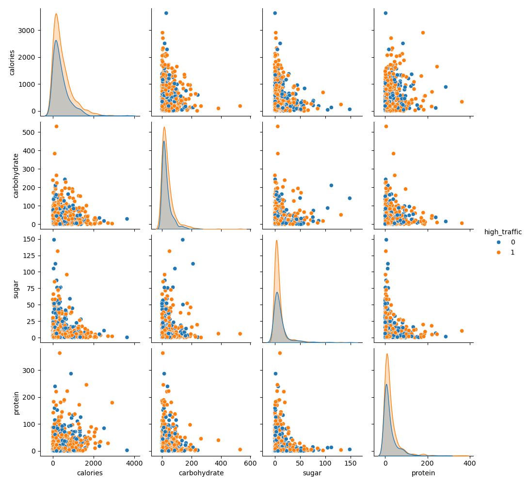
Pairplot showing relationships between numerical features and high_traffic categories.

Categorical Data Analysis

To further understand the distribution of categorical features across high_traffic categories, a countplot was generated. This visualization highlights how different recipe categories (e.g., Potato, Pork, Breakfast) are represented in both high-traffic and low-traffic groups.

• Vegetable and Potato Categories: These categories are more dominant in high-traffic recipes compared to others.
• Dessert and Beverages: These categories are less represented in high-traffic recipes.

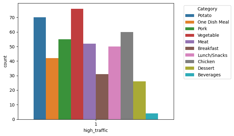
Countplot showing the distribution of recipe categories across high_traffic values.

---

Model Development

Overview

To predict recipe traffic, six machine learning models were trained and evaluated. Each model was optimized through hyperparameter tuning, ensuring the best possible performance on the validation set.

Models and Technical Details

1. Logistic Regression:
   • Purpose: A linear model suitable for binary classification tasks with interpretable coefficients.
   • Parameters:
     • Penalty: l2 (Ridge regularization) to prevent overfitting.
     • C: 1.0 (inverse regularization strength, tuned between 0.1 and 10).
     • Solver: liblinear (suitable for small to medium-sized datasets).
   • Optimization:
     • Standardized all numerical features to ensure coefficients are on the same scale.
2. Random Forest:
   • Purpose: An ensemble learning method combining multiple decision trees to reduce variance and overfitting.
   • Parameters:
     • Number of Trees: n_estimators = 100 (tuned in the range of 50–200).
     • Maximum Depth: max_depth = 10 (tuned to prevent overfitting).
     • Minimum Samples Split: min_samples_split = 5 (minimum number of samples required to split an internal node).
     • Criterion: gini (default for impurity-based splits).
   • Optimization:
     • Performed grid search over key hyperparameters.
     • Feature importance scores were extracted post-training.
3. K-Nearest Neighbors (KNN):
   • Purpose: A non-parametric method relying on proximity to predict class labels.
   • Parameters:
     • Number of Neighbors: n_neighbors = 5 (tuned between 3–15).
     • Distance Metric: minkowski with p=2 (equivalent to Euclidean distance).
     • Weights: uniform (all neighbors have equal weight).
   • Optimization:
     • Applied feature scaling (standardization) to ensure equal contribution from all numerical features.
     • Validation performance declined with higher k due to loss of local structure.
4. Support Vector Machine (SVM):
   • Purpose: A powerful linear classifier effective in high-dimensional spaces.
   • Parameters:
     • Kernel: rbf (Radial Basis Function) to capture nonlinear relationships.
     • Regularization Parameter: C = 1.0 (tuned between 0.1–10).
     • Gamma: scale (controls kernel influence, tuned between 0.001–1.0).
   • Optimization:
     • Used grid search to fine-tune hyperparameters.
     • Balanced class weights to address class imbalance.
5. Gradient Boosting:
   • Purpose: An ensemble method that builds trees sequentially, correcting previous errors.
   • Parameters:
     • Learning Rate: 0.1 (tuned between 0.01–0.3).
     • Number of Estimators: n_estimators = 100 (optimized for validation performance).
     • Maximum Depth: max_depth = 3 (controls complexity of individual trees).
     • Subsample: 0.8 (percentage of samples used for training each tree).
   • Optimization:
     • Early stopping based on validation loss to prevent overfitting.
6. Neural Networks:
   • Purpose: A multilayer perceptron (MLP) for capturing complex nonlinear relationships.
   • Architecture:
     • Input Layer: Matches the number of input features.
     • Hidden Layers: Two layers with 128 and 64 neurons, respectively.
     • Output Layer: Single neuron with sigmoid activation for binary classification.
   • Parameters:
     • Activation Function: ReLU for hidden layers.
     • Optimizer: Adam with learning rate 0.001.
     • Loss Function: Binary cross-entropy.
     • Batch Size: 32.
     • Epochs: 50 (with early stopping based on validation accuracy).
   • Optimization:
     • Used dropout (rate = 0.2) to mitigate overfitting.
     • Applied batch normalization for faster convergence.

Model Training Workflow

1. Data Splitting:
   • Training Set: 70%.
   • Validation Set: 15%.
   • Testing Set: 15%.
2. Cross-Validation:
   • Stratified 5-fold cross-validation was used to ensure balanced class distributions in all splits.
3. Hyperparameter Tuning:
   • Grid search and random search were employed to identify the best hyperparameters for each model.
   • Validation performance metrics (e.g., F1 Score and ROC AUC) guided parameter selection.
4. Performance Evaluation:
   • Each model was evaluated using the testing set to ensure unbiased performance estimates.

---

Performance Metrics

To evaluate each model, the following metrics were used:

• Precision: Proportion of true positive predictions among all positive predictions.
• Accuracy: Overall correctness of predictions.
• Recall: Proportion of true positives identified among all actual positives.
• F1 Score: Weighted average of precision and recall.
• ROC AUC Score: Measures the ability of the model to distinguish between classes.

Model Performance Comparison

Below is the performance comparison of the machine learning models evaluated:

Model	Precision	Accuracy	Recall	F1 Score	ROC AUC Score
Logistic Regression	0.789916	0.756345	0.803419	0.79661	0.83515
Random Forest	0.744186	0.725888	0.820513	0.780488	0.78734
K-Nearest Neighbor	0.601351	0.558376	0.760684	0.671698	0.534028
Support Vector Machine	0.803419	0.766497	0.803419	0.803419	0.830983
Gradient Boosting	0.742857	0.751269	0.888889	0.809939	0.803205
Neural Network	0.787611	0.736041	0.760684	0.773913	0.806838

The metrics include Precision, Accuracy, Recall, F1 Score, and ROC AUC Score to provide a comprehensive view of model performance.

Why Logistic Regression and Gradient Boosting?

Logistic Regression and Gradient Boosting stand out due to their robust performance across multiple evaluation metrics:

• Logistic Regression:
  • High precision (0.789) and ROC AUC score (0.835) indicate strong ability to correctly classify high-traffic recipes.
  • Simplicity and interpretability make it ideal for understanding feature contributions to predictions.
• Gradient Boosting:
  • Achieves the highest recall (0.889) among all models, effectively identifying recipes with high traffic.
  • Provides a balance between precision, recall, and F1 score, making it suitable for a range of applications.

Visualization of Performance

Confusion Matrices

The confusion matrix below demonstrates the classification performance of Logistic Regression and Gradient Boosting. These visualizations provide a breakdown of predictions for true positives, true negatives, false positives, and false negatives. The ROC curves evaluate the trade-off between sensitivity (True Positive Rate) and specificity (False Positive Rate) for the two best-performing models:

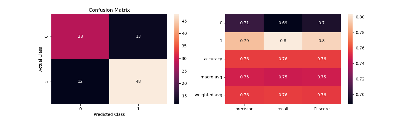Confusion matrix for Logistic Regression.

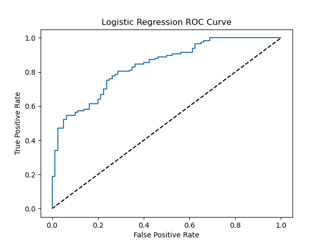
Receiver Operating Characteristic curve for Logistic Regression.

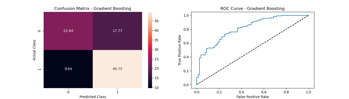Confusion matrix for Gradient Boosting.

---

Feature Importance

Key insights from feature importance analysis reveal the significant predictors for recipe traffic and user engagement. The following observations are based on the analysis of Logistic Regression and Gradient Boosting models:

Logistic Regression

• Vegetable: Emerged as the most critical feature, with a strong influence on recipe traffic. Recipes labeled with vegetables gained the highest user interaction.
• Potato: Demonstrated a notable contribution to engagement, highlighting its popularity in recipes.
• Pork and Meat: Ranked high, showing their relevance in driving traffic, especially for specific audience groups.
• Breakfast: Indicated as an essential predictor of recipe traffic, likely due to its broad appeal across users.

Gradient Boosting

• Protein: Identified as the most impactful feature in Gradient Boosting, highlighting its association with user interest and dietary preferences.
• Vegetable: Retained its significance, underscoring its universal appeal in recipe engagement.
• Breakfast: Consistently appeared as a critical category, reinforcing its importance in predicting recipe traffic.
• Recipe Attributes (Carbohydrate, Calories, Sugar): Demonstrated relevance, especially in health-conscious user segments.

Combined Observations

• Consistency Across Models: Features like Vegetable and Breakfast were consistently highlighted in both models, proving their significance across different predictive approaches.
• Distinctive Insights: Logistic Regression emphasizes categorical features (e.g., types of meals), while Gradient Boosting uncovers more nuanced associations with continuous attributes (e.g., protein, carbohydrates, and sugar).

Visualizations

1. 
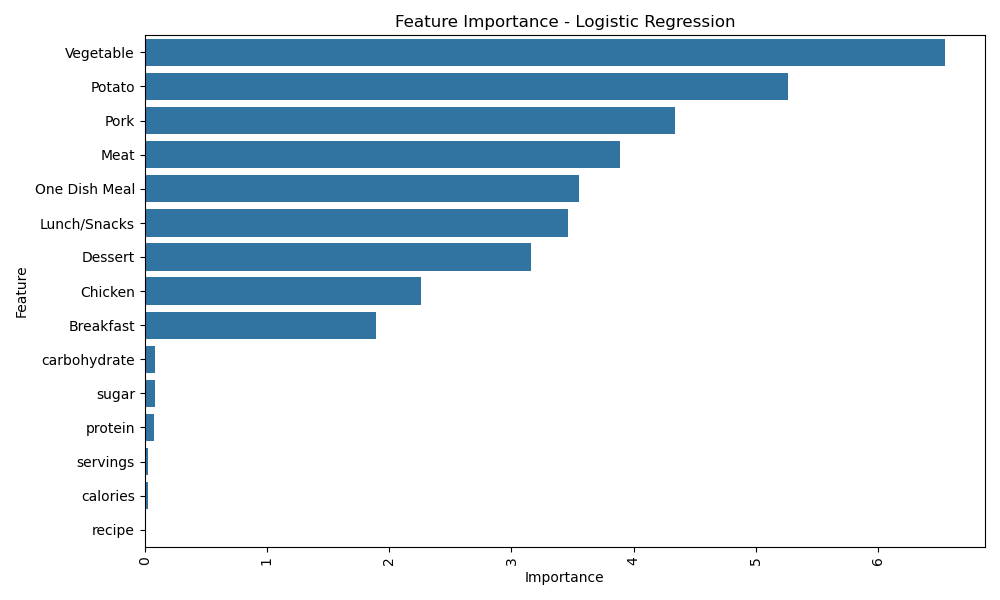
   Top features identified by Logistic Regression.

2. 
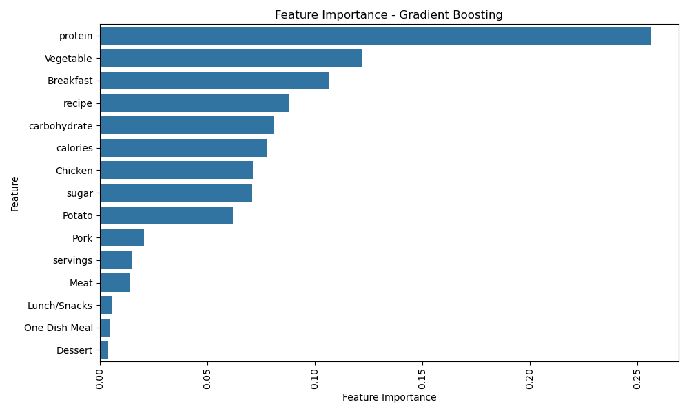
   Top features identified by Gradient Boosting.

By integrating insights from both models, this analysis provides a comprehensive understanding of the features driving recipe popularity and user engagement.

---

Conclusion

Key Takeaways

• Logistic Regression: Best-performing model due to its balance of precision, recall, and simplicity.
• Gradient Boosting: Provided strong performance, particularly for minority class predictions.
• Feature Importance: Nutritional features (e.g., protein) and categorical features (e.g., Breakfast) are strong drivers of recipe traffic.

Business Impact

• Insights from this analysis can help prioritize recipes with high traffic potential, optimize recipe recommendations, and increase overall user engagement.

Future Directions

1. Feature Engineering: Incorporate additional data points like preparation time, ingredient costs, and user ratings.
2. Advanced Models: Experiment with ensemble methods (e.g., stacking) for enhanced predictive performance.
3. Deployment: Integrate the model into a real-time recommendation system for recipe platforms.

---

Explore the Full Project

For detailed code, visualizations, and further insights, visit the GitHub Repository.

---